Statistical data analysis of NorCal's tire size video
Why am I doing this
First of all, I want to get it out of the way that I’m not “hating” on Jeff or his content, I actually like his channel quite a lot and have spent a lot hours watching his content. However, his latest videos, just like this one where he tests different tire sizes, are part of a trend of “bro-science” videos, which I see appearing a lot on YouTube lately. The intention is not malicious, but I think not enough nuance is giving about the statistical significance in these kind of videos. I think it should be made really clear that tests with such a limited sample size, are anecdotal at best. In this document, I’ll try to explain and prove why. I realize this blogpost might already be to advanced, but in my written text I try to explain things inituitivly, without the need for understanding or knowing all the math behind it.
The data
I extracted all the info of the tests ran by Jeff and Will into a data table. Original data from this video:
The data consists of 6 test runs, each tire size got tested twice at a different average power. I converted the time from minutes to seconds for easy of use. Tire size is in mm, Power in Watt and time in seconds.
data

## # A tibble: 6 × 3
##    Tire Power  Time
##   <dbl> <dbl> <dbl>
## 1    28   301   852
## 2    32   301   830
## 3    34   301   833
## 4    28   226   943
## 5    32   226   924
## 6    34   226   939
The analysis
A statistical analysis always starts (or at least should) with a question. What info do we want to retrieve from our data? In science, this question is ideally defined before doing the experiment. There even exist statistical tools that can help us determine the sample size we would need to detect certain differences at a statistically significant level, but that is a topic for another time.
In this case, we could formulate our question as: “Which tire size makes me go faster?” or, reformulated a bit more dry: ”Does tire size have a significant influence on time?“.
Analysis with a linear and quadratic model
First, we will try to answer this question using a model with linear and quadratic terms. Simply put, we will try to find a meaningful relationship between an outcome (in this case, the time) and certain explanatory variables, called this way because they explain part of the variation of the outcome (in this case, tire size and power). For this part of the analysis, we’ll treat all variables as continuous, numerical variables.
I won’t bother you with the math behind how this works and will try to keep it intuitively.
First, let’s plot our data points and explore the relationships visually.
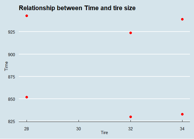
Visually, we can see that there seems the be a connection between tire size and time, however, it’s definitely not linear. What Jeff assumes in his video, and what can also slightly be seen here, is that there seems to be a quadratic relationship between tire size and time, leading to a U-shaped curve.
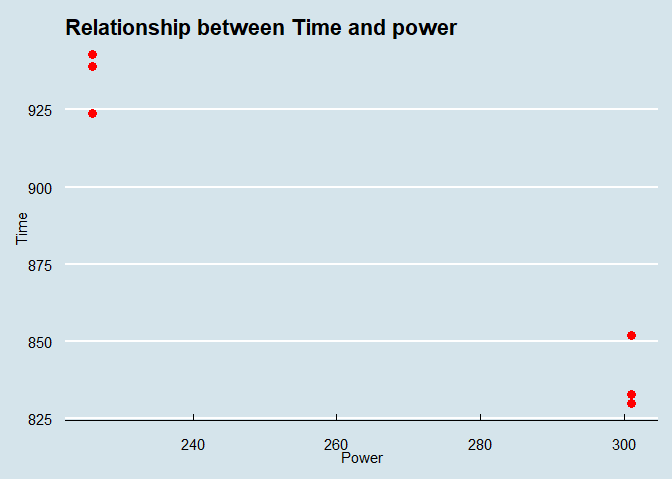
Visually, we can see that there seems the be a linear connection between power and time, more power yields a lower time spend on the bike (hooray!).
Now that we know what we are looking at, can we actually prove that this data is enough to make conclusions? Here is where we go further than just the visual interpretation of the data and go beyond the “science” done in Jeff’s video.
Let’s try to create a model that tries to explain time (Y, our response variable) using information from Tire size and Power (our explanatory variables) in the way we just observed: time has a linear relationship with power, and a quadratic relationship with tire size. We can then use the model to see if tire size is significantly explaining the variation of the time!
The model we will evaluate looks (simplified) like this:
Time = B0 + B1 x Power + B2 x Tire size + B3 x Tiresize^2
In order to create a model which we could use to predict new times, based on power and tire size, we need to estimate the terms B0, B1, B2 and B3. If you want to know how this is done mathematically, Google for “least squares regression”. For now, just think of it as a method that finds a way to fit a curve through are data that tries to minimize the error between the curve and the actual data points. In R, this is done with the lm() function, after which we can check the results using the summary() function.
##
## Call:
## lm(formula = Time ~ Power + Tire + Tire2, data = data)
##
## Residuals:
##    1    2    3    4    5    6
##  3.0  1.5 -4.5 -3.0 -1.5  4.5
##
## Coefficients:
##              Estimate Std. Error t value Pr(>|t|)
## (Intercept) 2819.1267   586.0640   4.810  0.04060 *
## Power         -1.2933     0.0611 -21.167  0.00222 **
## Tire        -101.3750    38.1948  -2.654  0.11746
## Tire2          1.6042     0.6187   2.593  0.12210
## ---
## Signif. codes:  0 '***' 0.001 '**' 0.01 '*' 0.05 '.' 0.1 ' ' 1
##
## Residual standard error: 5.612 on 2 degrees of freedom
## Multiple R-squared:  0.9957, Adjusted R-squared:  0.9892
## F-statistic: 153.8 on 3 and 2 DF,  p-value: 0.006466
All this info might look daunting, but let’s explain the gist of it. Because this is a quadratic model, it’s not always as easy to interpret what’s happening here, so for now, I’ll keep it short.
First, looking at power, our “suspicion” is confirmed. The estimated coefficient for power (B1) in our model is -1.3. This means, that if all other factors are kept constant, based on this data, an increase of power with 1 Watt will lead to a reduction in time of 1.3 seconds. Moreover, the stars indicate that this term is significant! That means that there is statistical proof to believe that we are pretty certain of this effect of power on time, even with this limited data!
Maybe by now you noticed that these stars are not appearing behind our two “Tire” explanatory variables. So both tire and tire size squared are not significantly explaining any of the variation in time in this dataset. Basically saying that, purely based on his gathered data, Jeff’s finding might as well been due to chance.
Adding a little bonus, we can take a look at the confidence intervals of these estimates of the coefficients. Basically, they give the range of the estimate for which we are 95% sure the estimate lies between those values.
##                   2.5 %      97.5 %
## (Intercept)  297.496975 5340.756359
## Power         -1.556230   -1.030437
## Tire        -265.714017   62.964017
## Tire2         -1.057964    4.266297
As you can see, the confidence interval for power is quite tight, and the estimate is always negative. You should read this as, “based on this data, I’m 95% sure that the time needed to complete the course will reduce between 1.03 and 1.55 seconds if I push 1 Watt harder”.
Ok, now that we established why Jeff should be a bit more careful in his conclusions (I really would love to go see him go full science mode and include enough repetitions of these experiments to get to a statistically significant level). Let’s cut him a bit more slack and try one more type of analysis.
Analysis with ANOVA using power and tire as categorical variables
ANOVA is short for “analysis of variance” and basically also is some sort of a linear model. Thus, what we want to do is analyze the variance of the time. For this part, let’s rephrase Jeff’s claim to “32mm tires are faster than 28 and 34mm tires independent of the power pushed”. So we reduce the problem to: were the 32mm tires faster, both in the high and low power test?
For this, we won’t consider the tire size and power as numerical variables, but as categorical variables, and see if the time differs significantly between the categories.
Again, let’s start by looking at the data.
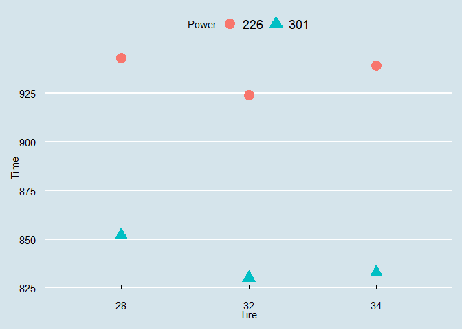
Now that we categorized our data, we again see the story Jeff is telling us: higher power yields a lower time (we agree!) and 32mm is the fastest at both low and high power (we don’t agree just yet!).
Now, let’s try and use the ANOVA method and see what we can learn from it’s output.
##             Df Sum Sq Mean Sq F value  Pr(>F)
## Power        1  14113   14113 448.048 0.00222 **
## Tire         2    422     211   6.704 0.12981
## Residuals    2     63      32
## ---
## Signif. codes:  0 '***' 0.001 '**' 0.01 '*' 0.05 '.' 0.1 ' ' 1
These results again confirm what we saw earlier. Based on this data, there is a significant difference in time between the observations at lower power, compared to high power, but there is no significant difference in time between the different sets of tires.
Finally, we can check the pairwise comparisons between the sets of tires. Here I applied the function TukeyHSD()
##   Tukey multiple comparisons of means
##     95% family-wise confidence level
##
## Fit: aov(formula = Time ~ Power + Tire, data = data)
##
## $Tire
##        diff       lwr      upr     p adj
## 32-28 -20.5 -53.56177 12.56177 0.1203606
## 34-28 -11.5 -44.56177 21.56177 0.3027699
## 34-32   9.0 -24.06177 42.06177 0.4146694
In the table you can see the pairwise comparisons between the different tire sizes and the estimated effect. You can also see the lower and upper boundary of the 95% confidence interval. However, these differences are deemed statistically insignificant (p adj is > 0.05). So again, based on this data, the 32 isn’t faster than the 28, neither is the 34.
Conclusion
Ok, so basically we did a lot of things to come to the conclusion: based on Jeff’s data, we can say that pushing the pedals harder makes you faster, but that we are uncertain of the effect of tire size. Of course, there is some truth in videos like this, and I really think Jeff has no ill intent and/or is being a shill for biking companies pushing wider tires. However, I do think it’s a slippery slope when videos like this are presented as “science” and “real results”, because they are most definitely not! I encourage content creators to put more effort in these things, maybe even consult some tutorials on statistics! I’m not saying they should be posting scientific research papers, but it will make it so much more reliable and informative if things like this are tested and analyzed properly! I hope with this blog post I sparked some interest in statistics among you, maybe you’ll end up Google-ing some of the stuff we did here! In any case, have fun cycling and be safe on the road!