Case study: targeted metabolite detection using TARDIS in cardiovascular disease

Introduction

TARDIS offers an easy and straightforward way to automatically calculate area under the peak, max intensity and various quality metrics for targeted chemical compounds in LC-MS data. It makes use of an established retention time correction algorithm from the xcms package and loads MS data as Spectra objects so it’s easily integrated with other tools of the Rformassspectrometry initiative.

See README for installation instructions.

In this vignette, a case study on publicly available biological data is described. We presume that we discovered a list of important metabolite biomarkers for cardiovascular disease (CVD), which we would like to validate in this dataset.

Dataset

We use the MetaboLights dataset MTBLS8735, an example untargeted metabolomics dataset tailored to quantify the small polar metabolome in human plasma samples and aimed to identify differences between individuals suffering from a cardiovascular disease (CVD) and healthy controls (CTR). The subset analyzed here includes data for three CVD patients, three CTR individuals, and four quality control (QC) samples. The QC samples, representing a pooled serum sample from a large cohort, were measured repeatedly throughout the experiment to monitor signal stability.

All samples were analyzed using ultra-high-performance liquid chromatography (UHPLC) (Agilent 1290; Agilent Technologies, Santa Clara, CA, USA) coupled to a Q-TOF mass spectrometer (TripleTOF 5600+; AB Sciex, Foster City, CA, USA). The chromatographic separation was based on hydrophilic interaction liquid chromatography (HILIC) and performed using an Acquity BEH amide, 100 x 2.1 mm column (Waters Corporation, Milford, MA, USA).

The list of internal standards: Alanine 13C315N (0.9 μg/mL), arginine 13C615N4 (1.8 μg/mL), aspartic acid 13C415N (1.3 μg/mL), cystine 13C615N2 (1.2 μg/mL), glutamic acid 13C515N (1.5 μg/mL), glycine 13C215N (0.8 μg/mL), histidine 13C615N3 (1.6 μg/mL), isoleucine 13C615N (1.3 μg/mL), leucine 13C615N (1.3 μg/mL), lysine 13C615N2 (1.5 μg/mL), methionine 13C515N (1.5 μg/mL), phenylalanine 13C915N (1.7 μg/mL), proline 13C515N (1.2 μg/mL), serine 13C315N (1.1 μg/mL), threonine 13C415N (1.2 μg/ mL), tyrosine 13C915N (1.8 μg/mL) and valine 13C515N (1.2 μg/mL).

For more details, we refer to the MetaboLights repository.

Loading data

The first step is creating a data.frame that describes the metabolites of interest. In this case, this are the internal standards and the 6 biomarkers of interest. Following columns at least need to be present for each compound:

A compound ID, a unique identifier
A compound Name
Theoretical or measured m/z
Expected RT (in minutes)
A column that indicates the polarity of the formed ion for that compound

Extra columns can be included in the file, but will be ignored by TARDIS unless otherwise indicated.

An input file (either .xlsx or .csv) can be converted to a correct data.frame using the createTargetList() function. Input parameters needed are: the path to the file, the patterns for positive and negative ionization, the polarity of interest, the columnn that contains the ionization mode and the other columns of interest.

library(readxl)
input <- read.csv2("vignette_data/bio_targets.csv",sep = ",")
kableExtra::kable(head(input))

ID	name	abbreviation	formula	POS	NEG	RT	data_set	sample	operator	version	quality_NEG	quality_POS	mz	mzmin	mzmax	rtmin	rtmax	rt
1	Carnitine (D3)	carnitine_d3	164.124	[M+H]+	NA	61	2019_11_matrix_effect	serum	Mar Garcia-Aloy	2	3_bad	2_medium	165.131276	165.126276	165.136276	51	71	1.016666667
2	Creatinine (N-Methhyl_D3)	creatinine_methyl_d3	116.0777	[M+H]+	[M-H]-	126	2019_11_matrix_effect	serum	Mar Garcia-Aloy	2	2_medium	2_medium	117.084976	117.079976	117.089976	116	136	2.1
3	Glucose (6,6-D2)	glucose_d2	182.0759	[M+Na]+	[M+CHO2]-	166	2019_11_matrix_effect	serum	Mar Garcia-Aloy	2	1_good	2_medium	205.06512	205.06012	205.07012	156	176	2.766666667
4	L-Alanine (13C3, 99%; 15N, 99%)	alanine_13C_15N	93.0548	[M+H]+	[M-H]-	167	2019_11_matrix_effect	serum	Mar Garcia-Aloy	2	2_medium	1_good	94.062076	94.057076	94.067076	157	177	2.783333333
5	L-Arginine HCl (13C6, 99%; 15N4, 99%)	arginine_13C_15N	184.1199	[M+H]+	[M-H]-	183	2019_11_matrix_effect	serum	Mar Garcia-Aloy	2	0_perfect	0_perfect	185.127176	185.122176	185.132176	173	193	3.05
6	L-Aspartic acid (13C4, 99%; 15N, 99%)	aspartic_13C_15N	138.048	[M+H]+	[M-H]-	179	2019_11_matrix_effect	serum	Mar Garcia-Aloy	2	1_good	1_good	139.055276	139.050276	139.060276	169	189	2.983333333

The target data.frame is created using createTargetList(). For more info on how to use the function, check the help page: ?createTargetList

Our biomarkers are defined as:

library(TARDIS)
targets <- createTargetList("vignette_data/bio_targets.csv",
                            pos_pattern = "+",
                            neg_pattern = "-",
                            polarity = "positive",
                            ion_column = "POS",
                            columns_of_interest = c("ID", "name", "mz", "rt"))
kableExtra::kable(targets[21:26,])

	ID	NAME	m/z	tr
21	21	Unknown_1	182.0749	34.83789
22	22	Caffeine	195.0877	32.65668
23	23	BENZYL METHYL SULFIDE	161.0400	162.13668
24	24	Anthranilic acid	138.0547	148.39599
25	25	Isoproturon	229.1299	181.08828
26	26	Unknown_2	560.3603	33.54917

Below we extract our dataset from the MetaboLigths database and load it as an MsExperiment object. For more information on how to load your data from the MetaboLights database, we refer to the MsIO vignette.

library(MsExperiment)
library(MsIO)
library(MsBackendMetaboLights)
param <- MetaboLightsParam(mtblsId = "MTBLS8735",
                           assayName = paste0("a_MTBLS8735_LC-MS_positive_",
                                              "hilic_metabolite_profiling.txt"),
                           filePattern = ".mzML")
lcms1 <- readMsObject(MsExperiment(),
                      param,
                      keepOntology = FALSE,
                      keepProtocol = FALSE,
                      simplify = TRUE)

lcms1
#> Object of class MsExperiment 
#>  Spectra: MS1 (17210) 
#>  Experiment data: 10 sample(s)
#>  Sample data links:
#>   - spectra: 10 sample(s) to 17210 element(s).

Simplifying the sampleData:

colnames(sampleData(lcms1)) <- c("sample_name", "spectraOrigin",
                                "metabolite_asssignment_file",
                                "source_name",
                                "organism",
                                "blood_sample_type",
                                "type", "age", "unit", "phenotype")

# Add "QC" to the phenotype of the QC samples
sampleData(lcms1)$phenotype[sampleData(lcms1)$sample_name == "POOL"] <- "QC"
sampleData(lcms1)$sample_name[sampleData(lcms1)$sample_name == "POOL" ] <- c("POOL1", "POOL2", "POOL3", "POOL4")
sampleData(lcms1)$type[sampleData(lcms1)$type == "pool"] <- "QC"

#  Add injection index column
sampleData(lcms1)$injection_index <- seq_len(nrow(sampleData(lcms1)))

sampleData(lcms1)[, c("spectraOrigin",
                     "phenotype", "sample_name", "type",
                     "injection_index")] |>
    kableExtra::kable(format = "pipe")

spectraOrigin	phenotype	sample_name	type	injection_index
FILES/MS_QC_POOL_1_POS.mzML	QC	POOL1	QC	1
FILES/MS_A_POS.mzML	CVD	A	experimental sample	2
FILES/MS_B_POS.mzML	CTR	B	experimental sample	3
FILES/MS_QC_POOL_2_POS.mzML	QC	POOL2	QC	4
FILES/MS_C_POS.mzML	CTR	C	experimental sample	5
FILES/MS_D_POS.mzML	CVD	D	experimental sample	6
FILES/MS_QC_POOL_3_POS.mzML	QC	POOL3	QC	7
FILES/MS_E_POS.mzML	CTR	E	experimental sample	8
FILES/MS_F_POS.mzML	CVD	F	experimental sample	9
FILES/MS_QC_POOL_4_POS.mzML	QC	POOL4	QC	10

IMPORTANT! The sample type column (indicating the QCs) has to be named type. and the column indicating the file has to be named spectraOrigin.

Screening mode

First, we perform a screening step to check if our targets are visible within our m/z and RT windows.

We can run screening mode using the argument screening_mode = TRUE in the tardisPeaks function.

For more details on the inputs of the function, please read the help page ?tardisPeaks

To limit the running time of this vignette, we limit the internal standard targets to five, which should be enough for good RT alignment, given their retention times span throughout most of the analysis. For more info on how to choose the right “housekeeping compounds” for RT alignment, we refer the reader to the xcms documentation.

L-Cystine (13C6, 99%; 15N2, 99%)
L-Methionine (13C5, 99%; 15N, 99%)
L-Glutamic acid (13C5, 99%; 15N, 99%)
L-Phenylalanine (13C9, 99%; 15N, 99%)
L-Serine (13C3, 99%; 15N, 99%)

subset <- targets[c(17,14,7,8,15,21:26),]

results <- tardisPeaks( lcmsData = lcms1, 
                        dbData = subset,
                        mass_range = NULL,
                        polarity = "positive",
                        output_directory = "vignette_data/output/case/screening/",
                        batch_positions = list(c(1,10)),
                        QC_pattern = "QC",
                        int_std_id = as.character(1:20),
                        screening_mode = TRUE)
#> Performing retention time correction using 5 peak groups.

The resulting EICs are saved in the output folder and can be inspected.

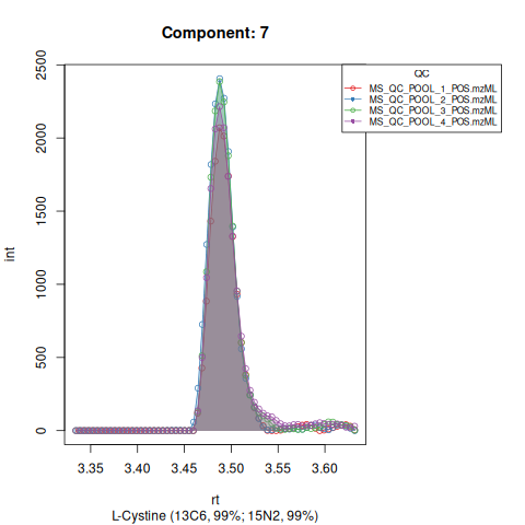
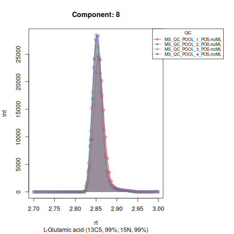
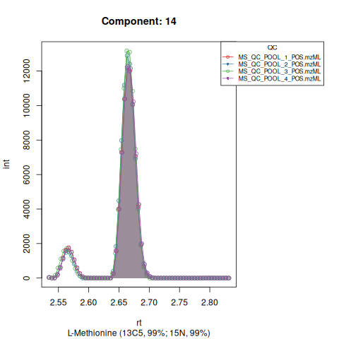
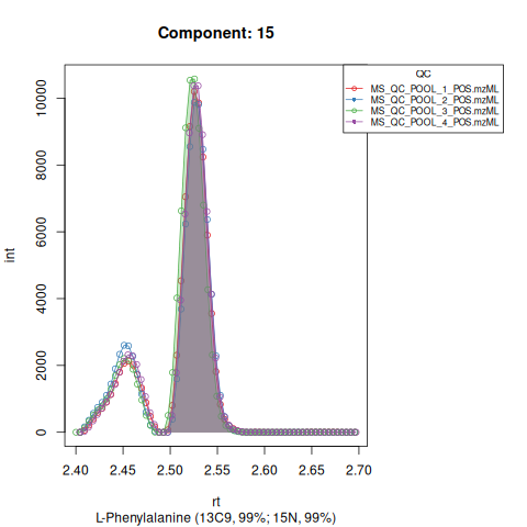
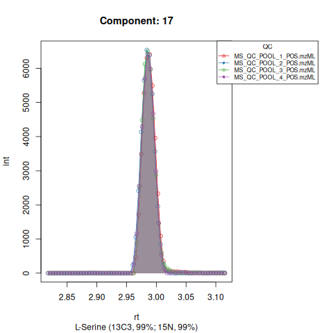
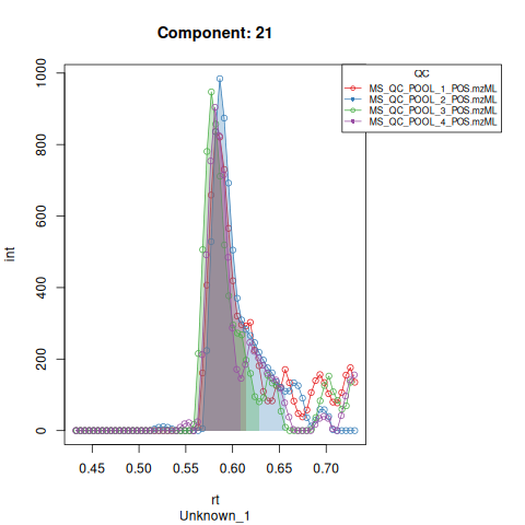
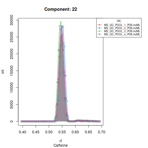
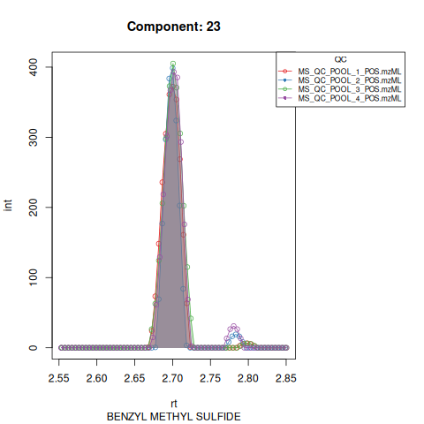
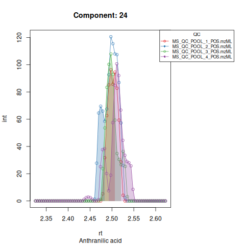
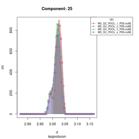
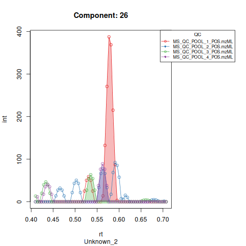
Based on the EICs we can see that detection, RT alignment and integration of target peaks in QC runs were successful. However, the signal of component 26, a non-annotated biomarker, is of remarkably lower quality than the others. One pooled QC shows a high signal that is absent in the other QC runs.

Peak detection

Now we can perform peak detection in all our runs by setting screening_mode = FALSE.

results <- tardisPeaks( lcmsData = lcms1, 
                        dbData = subset,
                        mass_range = NULL,
                        polarity = "positive",
                        output_directory = "vignette_data/output/case/",
                        batch_positions = list(c(1,10)),
                        QC_pattern = "QC",
                        int_std_id = as.character(1:20),
                        screening_mode = FALSE)
#> Performing retention time correction using 5 peak groups.
#> Aligning sample number 2 against subset ... OK
#> Aligning sample number 3 against subset ... OK
#> Aligning sample number 5 against subset ... OK
#> Aligning sample number 6 against subset ... OK
#> Aligning sample number 8 against subset ... OK
#> Aligning sample number 9 against subset ... OK

Results

The results object is a list that contains a data.frame with the AUC of each target in each run and a tibble that contains a feature table with the average metrics for each target in the QC runs.

AUC <- results[[1]]
kableExtra::kable(head(AUC))

Component	MS_A_POS.mzML	MS_B_POS.mzML	MS_C_POS.mzML	MS_D_POS.mzML	MS_E_POS.mzML	MS_F_POS.mzML	MS_QC_POOL_1_POS.mzML	MS_QC_POOL_2_POS.mzML	MS_QC_POOL_3_POS.mzML	MS_QC_POOL_4_POS.mzML
14	16525.69812	18002.5842	16543.549	17354.10495	19069.943	17914.6009	19826.2410	20773.350	21403.3610	20310.1275
15	17633.56844	18678.1921	16358.943	20086.53309	19134.836	11104.8497	18041.7061	17538.437	19005.3145	18484.4783
17	9696.06094	10009.2589	10862.924	9731.80795	10586.717	11158.9709	10348.6157	10773.937	10188.5909	10082.6647
21	NA	3573.0464	3157.537	47.03151	4260.996	NA	1498.4509	2006.222	1746.3844	1378.9488
22	827.47100	79504.3672	116928.037	2204.12719	166453.150	827.6966	36758.7755	40199.217	39582.0053	39544.2507
23	28.60398	384.4481	632.872	NA	1976.859	NA	660.7771	536.172	715.3061	672.9312

feat_table <- results[[2]]
kableExtra::kable(head(feat_table))

Component	AUC	MaxInt	SNR	peak_cor	foundRT	pop	ID	NAME	m.z	tr	mean	na.rm	trold
14	20578.2698	12635.3442	16.64761	0.9696404	159.81106	18.00	14	L-Methionine (13C5, 99%; 15N, 99%)	156.0722	159.81106	159.81106	TRUE	161.00000
15	18267.4839	10256.7736	12.89131	0.9476993	151.52398	21.25	15	L-Phenylalanine (13C9, 99%; 15N, 99%)	176.1135	151.52398	151.52398	TRUE	153.00000
17	10348.4520	6464.6150	19.84894	0.9757596	179.14857	17.50	17	L-Serine (13C3, 99%; 15N, 99%)	110.0570	179.14857	179.14857	TRUE	178.00000
21	1657.5015	918.1422	12.93310	0.9439880	34.89898	15.75	21	Unknown_1	182.0749	34.89898	34.89898	TRUE	34.83789
22	39021.0621	27834.8161	30.26548	0.9887586	32.87623	14.00	22	Caffeine	195.0877	32.87623	32.87623	TRUE	32.65668
23	646.2966	392.2353	17.00577	0.9647597	162.04193	14.50	23	BENZYL METHYL SULFIDE	161.0400	162.04193	162.04193	TRUE	162.13668

Other results include tables with the other metrics (Max. Int., SNR, peak_cor and points over the peak) and are saved into the output folder in .csv format.

maxint <- read.csv("vignette_data/output/case/int_table.csv",check.names = FALSE)[,-1]
SNR <- read.csv("vignette_data/output/case/snr_table.csv",check.names = FALSE)[,-1]
peak_cor <- read.csv("vignette_data/output/case/peakcor_table.csv",check.names = FALSE)[,-1]
pop <- read.csv("vignette_data/output/case/pop_table.csv",check.names = FALSE)[,-1]

kableExtra::kable(head(pop))

Component	MS_A_POS.mzML	MS_B_POS.mzML	MS_C_POS.mzML	MS_D_POS.mzML	MS_E_POS.mzML	MS_F_POS.mzML	MS_QC_POOL_1_POS.mzML	MS_QC_POOL_2_POS.mzML	MS_QC_POOL_3_POS.mzML	MS_QC_POOL_4_POS.mzML
14	21	22	26	25	19	20	19	18	17	18
15	23	22	25	23	24	23	21	21	22	21
17	16	20	14	15	15	14	17	18	19	16
21	NA	13	20	7	13	NA	13	21	17	12
22	10	14	13	13	14	9	15	14	14	13
23	7	12	11	NA	23	NA	15	12	16	15

Exploratory data analysis

The next section of this vignette describes an example exploratory data analysis using the results of TARDIS preprocessing.

PCA

First, we use perform a principal component analysis (PCA) using the AUC’s of our biomarkers:

# Load required packages
library(dplyr)
library(tidyr)
library(ggplot2)
# Limit input data to biomarkers and not ISTD targets
data <- AUC[4:9,]
sampledata <- data.frame(sampleData(lcms1))
# Remove "FILES/" prefix
sampledata$spectraOrigin <- gsub("FILES/", "", sampledata$spectraOrigin)
# Ensure row names correspond to Feature ID
rownames(data) <- data[, 1]
data <- data[, -1]  # Remove the feature ID column for PCA
# Transpose the data so that samples are rows and features are columns
data_t <- as.data.frame(t(data))
# Impute NA values
na_unidis <- function(z) {
    na <- is.na(z)
    if (any(na)) {
        min = min(z, na.rm = TRUE)
        z[na] <- runif(sum(na), min = min/2, max = min)
    }
    z
}
tmp <- apply(data_t, MARGIN = 1, na_unidis)
data_t <- t(tmp)
# Perform PCA
pca_result <- prcomp(data_t, scale. = TRUE,center = TRUE)
# Extract PCA scores
pca_df <- as.data.frame(pca_result$x)
pca_df$Sample <- rownames(pca_df)
# Merge with sample metadata to get phenotype information
pca_df <- left_join(pca_df, sampledata, by = c("Sample" = "spectraOrigin"))
# Plot PCA
ggplot(pca_df, aes(x = PC1, y = PC2, color = phenotype)) +
  geom_point(size = 3) +
  theme_minimal() +
  labs(title = "PCA",
       x = "Principal Component 1",
       y = "Principal Component 2") +
  scale_color_manual(values = c("red", "blue", "green")) # Customize colors if needed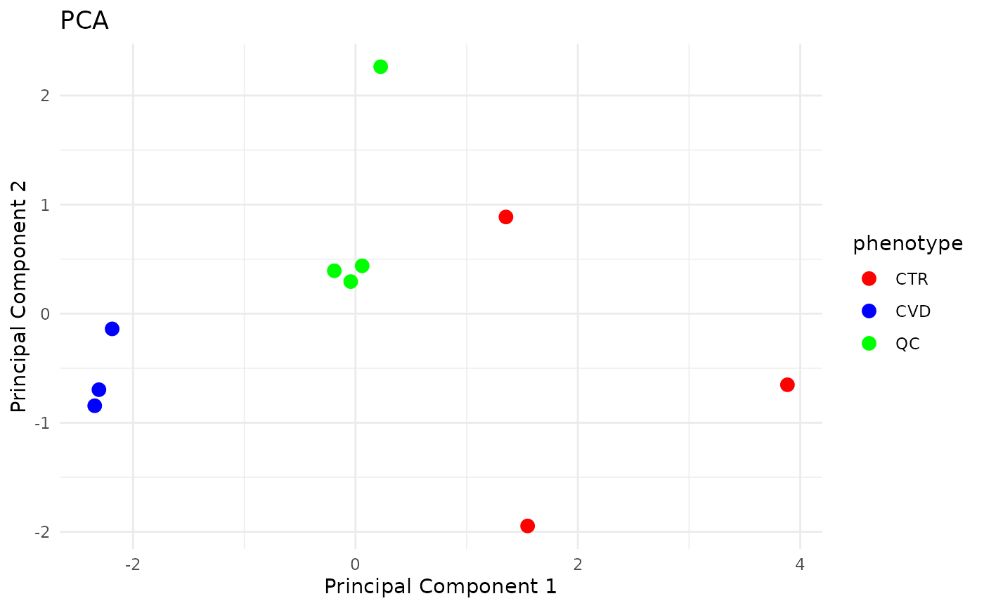

Results are as expected:

QC samples cluster together, indicating little technical variance in the analysis. However, one QC sample clearly differs from the others. This is due to component 26, which, as shown earlier, showed a large peak in one of the QC runs, but not in the others.
Samples with the CVD phenotype cluster together, more so than the CTR samples indicating that the biomarkers vary less within in the CVD phenotype as compared to the healthy controls.

Disregarding component nr 26, the PCA looks like:

# Limit input data to biomarkers and not ISTD targets
data <- AUC[4:8,]
sampledata <- data.frame(sampleData(lcms1))
# Remove "FILES/" prefix
sampledata$spectraOrigin <- gsub("FILES/", "", sampledata$spectraOrigin)
# Ensure row names correspond to Feature ID
rownames(data) <- data[, 1]
data <- data[, -1]  # Remove the feature ID column for PCA
# Transpose the data so that samples are rows and features are columns
data_t <- as.data.frame(t(data))
# Impute NA values
na_unidis <- function(z) {
    na <- is.na(z)
    if (any(na)) {
        min = min(z, na.rm = TRUE)
        z[na] <- runif(sum(na), min = min/2, max = min)
    }
    z
}
tmp <- apply(data_t, MARGIN = 1, na_unidis)
data_t <- t(tmp)
# Perform PCA
pca_result <- prcomp(data_t, scale. = TRUE,center = TRUE)
# Extract PCA scores
pca_df <- as.data.frame(pca_result$x)
pca_df$Sample <- rownames(pca_df)
# Merge with sample metadata to get phenotype information
pca_df <- left_join(pca_df, sampledata, by = c("Sample" = "spectraOrigin"))
# Plot PCA
ggplot(pca_df, aes(x = PC1, y = PC2, color = phenotype)) +
  geom_point(size = 3) +
  theme_minimal() +
  labs(title = "PCA",
       x = "Principal Component 1",
       y = "Principal Component 2") +
  scale_color_manual(values = c("blue", "red", "green")) # Customize colors if needed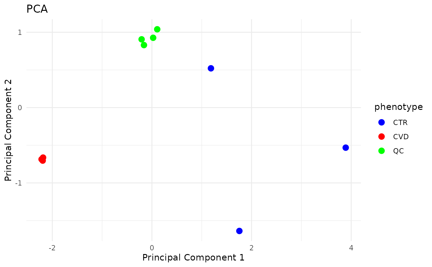

Differential abundance analysis

In this section we perform differential abundance analysis to investigate which differences in abudance of biomarkers we observe between the two phenotype groups.

First we remove the ISTD targets from the data and impute missing values.

# Limit input data to biomarkers and not ISTD targets
data <- AUC[4:8,]
sampledata <- data.frame(sampleData(lcms1))
sampledata$spectraOrigin <- gsub("FILES/", "", sampledata$spectraOrigin)
# Ensure row names correspond to Feature ID
rownames(data) <- data[, 1]
data <- data[, -1]  # Remove the feature ID column for PCA
data_t <- as.data.frame(t(data))
na_unidis <- function(z) {
    na <- is.na(z)
    if (any(na)) {
        min = min(z, na.rm = TRUE)
        z[na] <- runif(sum(na), min = min/2, max = min)
    }
    z
}
#' Row-wise impute missing values and add the data as a new assay
tmp <- apply(data_t, MARGIN = 1, na_unidis)
data_t <- as.data.frame(t(tmp))
# Merge with sample metadata
data_t$Sample <- rownames(data_t)
data_t <- left_join(data_t, sampledata, by = c("Sample" = "spectraOrigin"))
data_t <- data_t[-which(data_t$phenotype == "QC"),]

Next we visualize the log2 transformed abudances of each feature in each group using boxplots.

boxdata <- data_t[,c(1:5,15)]
boxdata <- pivot_longer(boxdata,cols = !phenotype,names_to = "feature",values_to = "abundance")
ggplot(boxdata, aes(x=feature, y=log2(abundance), fill=phenotype)) + 
    geom_boxplot() +
  scale_fill_manual(values = c("blue","red"))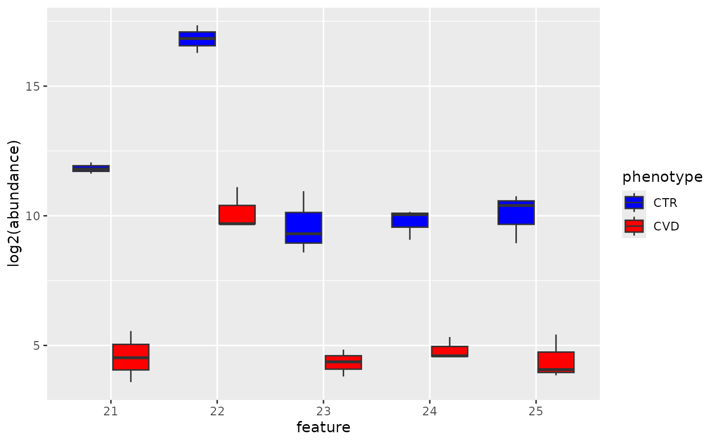

To test the differences for each biomarker, we use to wilcox.test function. From the boxplots above, we known that the biomarkers are underrepresented in the CVD phenotype, hence, we use the alternative = "less" option in the wilcox.test function. Data is log2 transformed.

pres <- data.frame(Feature = colnames(data_t)[1:5], p_value = NA)
for (i in 1:5) {
  feature_values <- data_t[, i]
  group1 <- log2(feature_values[data_t$phenotype == "CVD"])
  group2 <- log2(feature_values[data_t$phenotype == "CTR"])
  pres$p_value[i] <- wilcox.test(group1, group2,alternative = "less")$p.value
  }
pres$adj_p_value <- p.adjust(pres$p_value, method = "fdr")
knitr::kable(pres)

Feature	p_value	adj_p_value
21	0.05	0.05
22	0.05	0.05
23	0.05	0.05
24	0.05	0.05
25	0.05	0.05

Conclusion

Based on the results preprocessed using TARDIS, we can conclude that the earlier discovered metabolites are indeed valid biomarkers for the CVD phenotype and are significantly underrepresented in the CVD samples.

Pablo Vangeenderhuysen

2025-10-24